Theo Verelst Local Diary Page 63
I've ditched the usual header for the
moment, I think it doesn't help much anyhow.
This page is copyrighted by me, and may be read and transfered by any
means only as a whole and including the references to me. I
guess thats normal, the writer can chose that of course, maybe
I´ll make some creative commons stuff one day, of course I have
made Free and Open Source software and even hardware designs available!
This
page is under contruction, so check back later, too.
Mon Dec 29 12:54, 2008
Of course you don't NEED to use an full HD screen to view this page,
but it sure helps...
90s hits?
"When I'm walking through a shadow of Death and take a look at my
life..."
Billboard Hot 100 (1995)
Billboard Hot 100 (1998)
- 1. Too Close - Next
- 2. The Boy Is Mine - Brandy & Monica
- 3. You're
Still The One - Shania Twain
- 4. Truly
Madly Deeply - Savage Garden
- 5. How Do I
Live - LeAnn Rimes
- 6. Together
Again - Janet
- 7. All My Life - K-Ci & JoJo
- 8. Candle In
The Wind 1997 - Elton John
- 9. Nice & Slow - Usher
- 10. I Don't
Want To Wait - Paula Cole
- 11. How's It
Going To Be - Third Eye Blind
- 12. No, No, No - Destiny's Child
- 13. My Heart
Will Go On - Celine Dion
- 14. Gettin' Jiggy Wit It - Will Smith
- 15. You Make Me Wanna... - Usher
- 16. My Way - Usher
- 17. My All
- Mariah Carey
- 18. The First Night - Monica
- 19. Been Around The World - Puff Daddy & The Family
- 20. Adia - Sarah McLachlan
- 21. Crush
- Jennifer Paige
- 22. Everybody (Backstreet's Back) - Backstreet Boys
- 23. I Don't
Want To Miss A Thing - Aerosmith
- 24. Body Bumpin Yippie-Yi-Yo - Public Announcement
- 25. This
Kiss - Faith Hill
- 26. I Don't
Ever Want To See You Again - Uncle Sam
- 27. Let's Ride - Montell Jordan
- 28. Sex And Candy - Marcy Playground
- 29. Show Me Love - Robyn
- 30. A Song For Mama - Boyz II Men
- 31. What You Want - Mase
- 32. Frozen - Madonna
- 33. Gone Till November - Wyclef Jean
- 34. My Body - Lsg
- 35. Tubthumping - Chumbawamba
- 36. Deja Vu (Uptown Baby) - Lord Tariq & Peter Gunz
- 37. I Want You Back - 'N Sync
- 38. When The Lights Go Out - Five
- 39. They Don't Know - Jon B.
- 40. Make Em' Say Uhh! - Master P
Awfull.
A CUDA accelerated Cinelerra plugin
PPM 256
ICC profiles / prefs
After solving more than a handfull of bugs I had cinepaint running from
my own compilation.
The next thing after having compiled, added to and analysed here and
there the Cuda examples should be I thought to add some Cuda processing
to a slow plugin.
See also the NVidia Cuda forum.
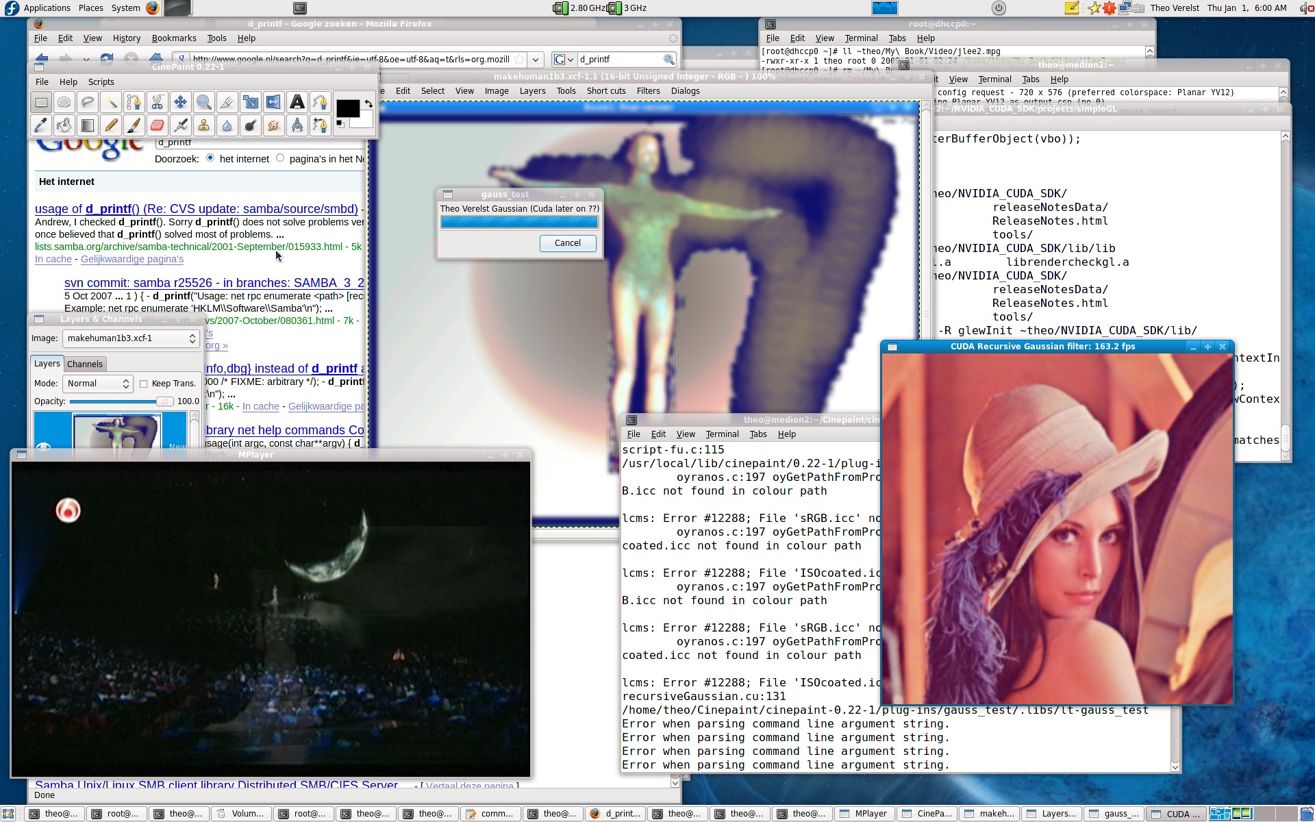
The first (actually) Cuda Cinepaint plugin ttyout screendump
The working Gaussian Blur Cuda plugin in Cinepaint:
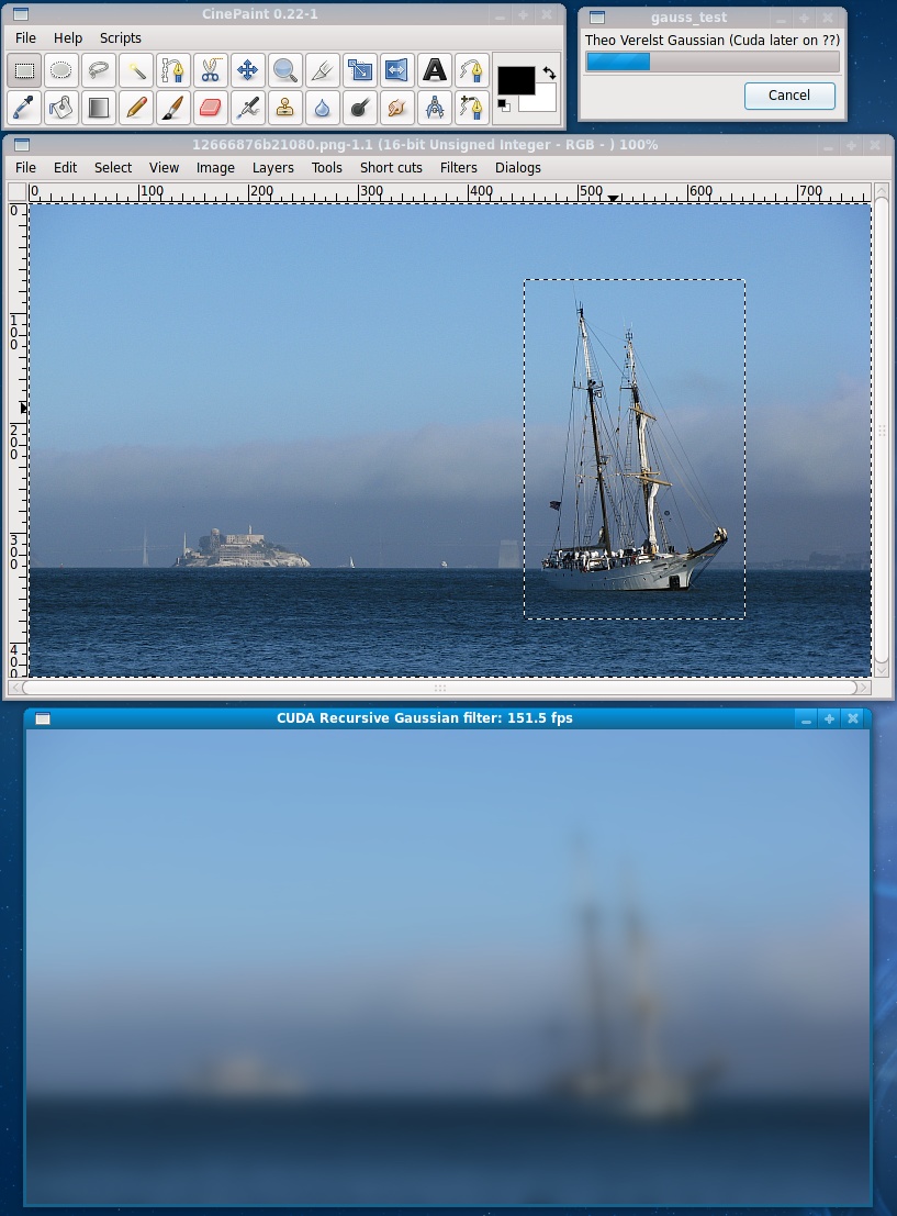
Is that 151.5 FRAMES PER SECOND ?! It is...
The result:

More compile work
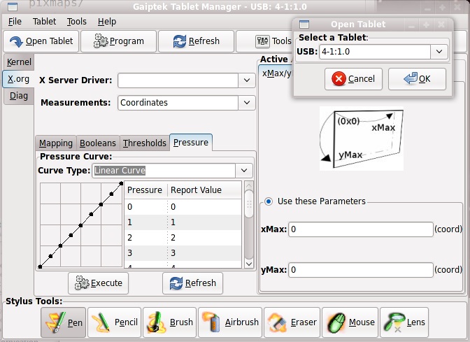
This don't compile/work on Fedora 10/64, Theo! Tell me about it, but
after many hours, this developer can make
it so. But, now the X driver needs work to talk nicely with it. Grrr.
Math for years of hand-computation
This was EE first year material in 1984 (magical year) at DUT when
elektisch was maybe still electrisch, I don't remember, but it was just
after the curriculum had been made into university level instead of
'hogeschool' which was kind enhanced bachelor level.
Taylor expansion means a differentiable function is replaced by a sum
of a number of polynomial terms, up til a certain degree, which are
computed by approximating a number of derivatives of the function at
that point. See mathematical literature for the rifht formulas. For
engineers such expansion is usefull because it is a good approximation
and the next term of the expansion of a certain degree is a upper bound
for the error, under certain strict conditions, which makes it a good
approximating expansion because it also is fairly stable and usable for
many physically oriented applications.
Here are some Maxima formulas and the result of giving them to that
package as assignment.
First a tryout of the taylor row of the 8th degree from Maxima:
taylor(exp(-x^2), x, 0, 8);
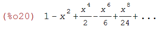
In fact it remembers its an expansion, but it only show the first 8
degree terms.
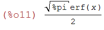
An important function in Physics and statistics is the gaussian, which
is not easy to integrate but maxima can do a formal integration with
filled in boundaries. Here is the formal integral with a built in
function (exercise: fill in the boundaries):
integrate(exp(-x^2),x);
Now I take a 200 (very many) degree taylor expansion of the gaussian
and integrate the Taylor expansion, which is possible because it's a
200 degree polynomial of even a decent form:
integrate([taylor(exp(-x^2),x,0,200)],
x, 0, 1000);
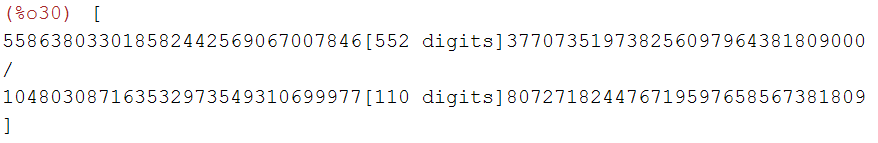
Notice that equalling fractions by maxima and working with
'infinite' precision numbers makes the resulting fraction which
aproximates the above integral have more than 500 digits!
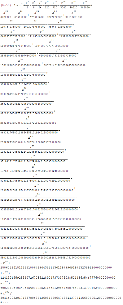
See below for a 100 term expansion (without integrating) in a smaller
form:
taylor(exp(-x^2),x,0,100);
This is a plot of the taylor expansion of the gaussian around 0:
plot2d([taylor(exp(-x^2),x,0,200)],
[x,-4,4], [plot_format, gnuplot]);
And of the derivative of the actual gaussian:
Now a plot of the difference between the gaussian and its 100th order
taylor expansion, plotting the approximation error between -5 and +5:
plot2d([taytorat((taylor(exp(-x^2),x,0,100)))-exp(-x^2)],
[x,-5,5],
[plot_format, gnuplot]);
We can see the approximation suddenly becomes very inaccurate above 4.7.
If we scale that graph down to look at the small errors when this
begins, we get for a 200 degree appoximation:
plot2d([taytorat((taylor(exp(-x^2),x,0,200)))-exp(-x^2)],
[x,-4,4],
[plot_format, gnuplot]);
But is this the result we're looking for ?! Where does the rounding
take place? Those are important questions I worked on.
The Guitar Rack of Choise ?
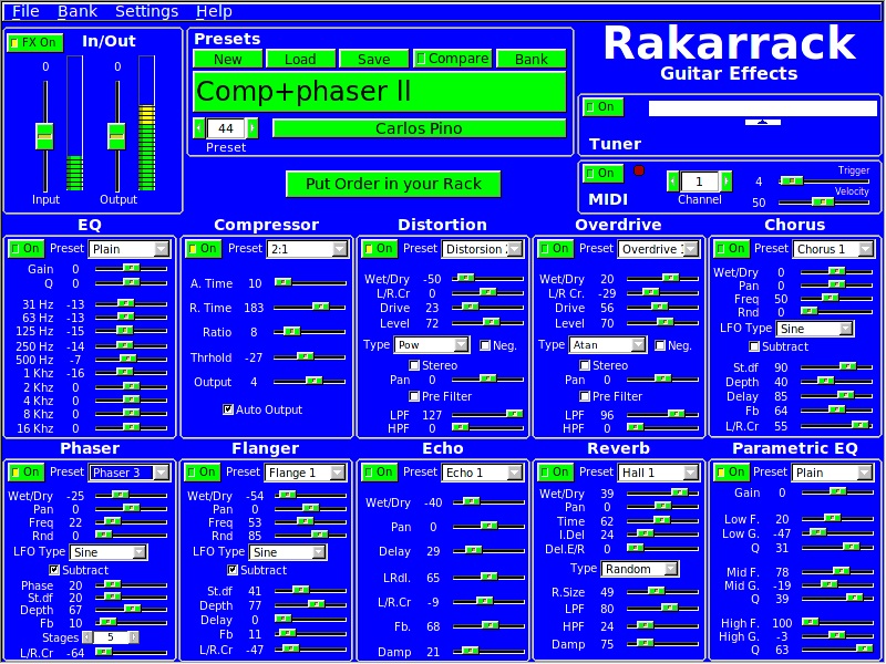
rakarrack 0.2.0 - Copyright (c) Daniel Vidal - Josep Andreu - Hernan
Ordiales
Heaeaeavvvyyy!